References

• Algorithmic Regularization in Learning Deep Homogeneous Models: Layers are Automatically Balanced, Simon S. Du, Wei Hut, Jason D. Lee (2018)
• The geometry of the deep linear network, Govind Menon (2024)

Two Key Problems

• Supervised Learning: Adjust the weights of a deep neural network so its predictions match the targets in a dataset as closely as possible.
• Matrix Factorization: Given a target matrix, find two smaller matrices whose product closely approximates the target.

Both problems are solved using gradient-based optimization

The Learning Problem: Goal & Model

1. Goal: Learn a function $f: \mathcal{X} \to \mathcal{Y}$ from a dataset of input-output pairs $\mathcal{D} = \{(x_i, y_i)\}_{i=1}^m$.
2. Model: We use a deep neural network, parameterized by weights $\mathbf{W}$, as our function approximator, $f(x; \mathbf{W})$.

The Learning Problem: Loss Function

3. Loss: We quantify prediction error using a loss function:

The Learning Problem: Optimization

4. Optimization: We find the best weights by minimizing the loss using the continuous-time dynamics of Gradient Flow.

Gradient Flow: Key Equation

Questions

• Convergence guarantees?
• Convergence rate?
• Non-convex case: Characterize the minimizer reached
• Effect of noise due to floating point errors, etc?

Our Focus: Deep Homogeneous Models

• A feed-forward neural network computes a function: \[ f(x; \mathbf{W}) = W^{(N)} \phi(\cdots \phi(W^{(1)}x)\cdots) \]
• We focus on networks where the activation function $\phi$ is homogeneous.

A Key Property: Homogeneity

An activation function $\phi$ is homogeneous of degree 1 if for any scalar $c > 0$:

• This property holds for many popular activations:
  • Linear: $\phi(z) = z$
  • ReLU: $\phi(z) = \max(0, z)$
  • Leaky ReLU: $\phi(z) = \max(az, z)$ for $0 < a < 1$
• It does not hold for functions like Sigmoid or Tanh.

The Consequence: Scale Invariance

Homogeneity in activations leads to a scale invariance in the entire network. We can scale up one layer's weights and scale down the next, and the overall function remains unchanged.

This is because the scalar $c$ passes through the homogeneous activation $\phi$ and cancels out.

The Optimization Puzzle

This scale invariance creates a fundamental problem for optimization:

• Non-uniqueness: If we find one good set of weights, there are infinitely many other sets that are just as good. \[ \left(W^{(i)}, W^{(i+1)}\right) \text{ is equivalent to } \left(cW^{(i)}, \frac{1}{c}W^{(i+1)}\right) \]
• Unboundedness: We can make the norm of the weights arbitrarily large (by choosing a large $c$) without changing the loss. \[ \|cW^{(i)}\|_F \to \infty \text{ as } c \to \infty \]

Why Classical Theory Fails

Many classical theorems that guarantee convergence of optimization algorithms rely on assumptions that are violated here.

• In deep homogeneous models, the loss landscape has "valleys" extending to infinity where the loss is low.
• The parameter iterates are not guaranteed to stay in a bounded region, making convergence analysis extremely difficult.

The "Obvious" Fix: Explicit Regularization

For a deep network, the most common form of explicit regularization is L2 regularization, also known as weight decay:

• This regularizer penalizes large weights in any layer, discouraging norms from becoming excessively large.
• This makes the objective coercive (the loss grows as weights increase), ensuring the parameters remain in a bounded set where analysis is more straightforward.

Matrix Factorization

The objective is to find factors $U \in \mathbb{R}^{d_1 \times r}$ and $V \in \mathbb{R}^{d_2 \times r}$ that approximate a target matrix $M^* \in \mathbb{R}^{d_1 \times d_2}$ where the rank $r \ll \min(d_1, d_2)$.

• This model is homogeneous: for any $c > 0$, the function is unchanged if we replace $(U, V)$ with $(cU, \frac{1}{c}V)$.
• The weights can become unbalanced and grow infinitely large.

The "Obvious" Fix: Explicit Regularization

A common theoretical workaround is to add a penalty term to the loss that forces the norms of the layers to be balanced:

• This regularizer removes the homogeneity and forces $\|U\|_F \approx \|V\|_F$.
• The modified objective is now "well-behaved" (e.g., coercive), and standard theory can be applied to prove convergence.

But... Is It Necessary?

Let's compare Gradient Descent on the original vs. the regularized problem. (Fig 1a from Du et al. 2018)

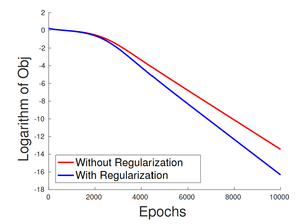
The convergence rates are competitive. The original, unregularized problem converges just fine.

The Empirical Surprise

What happens to the norms of the factors during training? (Fig 1b from Du et al. 2018)

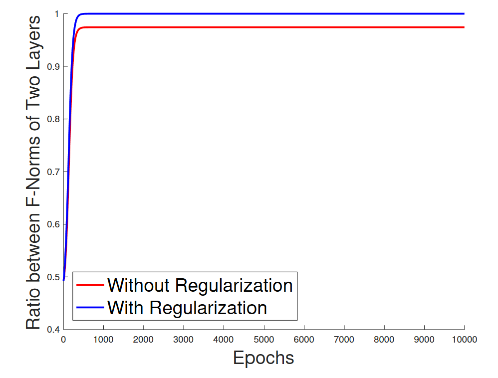
The ratio of the norms remains constant, even for the unregularized objective. The layers stay balanced on their own!

The Empirical Surprise

Similar observation for the Deep Linear Networks (DLN) (Fig 2 from Du et al. 2018)

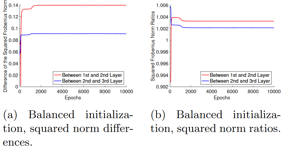
The ratio of the norms remains constant, even for the unregularized objective. The layers stay balanced on their own!

The Answer: Implicit Regularization

• The combination of the over-parameterized, homogeneous model structure and first-order optimization methods leads to a hidden property: Implicit Regularization.

The Answer: Implicit Regularization

• The combination of the over-parameterized, homogeneous model structure and first-order optimization methods leads to a hidden property: Implicit Regularization.
• The optimization dynamics on these models implicitly enforce a constraint that keeps the layer norms balanced.

The Answer: Implicit Regularization

• The combination of the over-parameterized, homogeneous model structure and first-order optimization methods leads to a hidden property: Implicit Regularization.
• The optimization dynamics on these models implicitly enforce a constraint that keeps the layer norms balanced.
• This prevents the parameters from running off to infinity in an unbalanced way.

Let's Formalize: Gradient Flow

To analyze this, we study the dynamics of Gradient Descent in the continuous-time limit.

The weights $\mathbf{W}$ evolve over time $t$ according to the differential equation:

This captures the behavior of GD with an infinitesimally small learning rate.

Corollary: Layer-wise Balancing

By summing over all neurons in a layer, we get a direct consequence for the entire weight matrices.

The Implication

The difference in squared norms between adjacent layers is constant over time.

• This explains the empirical observation!
• If we initialize the network with weights that are balanced (i.e., $\|W^{(h)}(0)\|_F^2 = \|W^{(h+1)}(0)\|_F^2$), they will remain balanced for all time.
• Common initialization schemes like Xavier or Kaiming initialization do precisely this. They set the initial norms to be roughly equal. (More on "roughly equal" later)

A Stronger Invariance for Linear Networks

For the special case of linear activations ($\phi(x)=x$), an even stronger, matrix-level quantity is conserved.

This shows that not just the difference of squared norms, but a more structured matrix difference, remains constant throughout training.

Connecting to Matrix Factorization

The matrix factorization problem for $UV^T \approx M^*$ is equivalent to a 2-layer linear network with weights $W^{(1)} = V^T$ and $W^{(2)} = U$.

Applying the stronger invariance from Theorem 2.2 to this case (with $h=1$) tells us that the quantity

is conserved under gradient flow.

This implies that if we initialize with $U_0^T U_0 = V_0^T V_0$, this balance will be maintained by the dynamics.

From Theory to Practice: Open Questions

Gradient flow with perfectly balanced initialization is an idealization. In practice, we face a more complex scenario:

• What happens if the initialization isn't perfectly balanced?
• How does the discrete nature of Gradient Descent (with $\eta > 0$) affect the autobalancing property?
• Can we prove convergence to a global minimum for these unregularized problems?

Answers for Matrix Factorization (Rank-r)

While these questions are difficult for general deep networks, for the matrix factorization problem, we have concrete answers.

This shows that the balancing property of gradient flow approximately holds for gradient descent.

Stronger Results for Rank-1 Case

For the rank-1 problem, even stronger results hold, guaranteeing not just balance but also fast convergence.

This provides a comprehensive answer for the simplest non-trivial homogeneous model.

Proof Setup: Two Linear Layers

To see the core idea, we'll prove the autobalancing result for the simplest case: a two-layer linear network.

• Consider the function $x_{out} = W_2 W_1 x_{in}$.
• The loss $\mathcal{L}$ is some function of the output, $L(x_{out})$.
• The weights evolve under gradient flow: $\frac{d}{dt}W_1 = -\nabla_{W_1}\mathcal{L}$ and $\frac{d}{dt}W_2 = -\nabla_{W_2}\mathcal{L}$.

The Goal

We want to prove the stronger, layer-wise balancing property that holds for linear networks (Theorem 2.2).

(Note: For matrices, $W W^T$ and $W^T W$ are SPSD matrices that capture the geometry of the rows and columns, respectively.)

Tool: Backpropagation (Chain Rule)

First, we write down the gradients using the chain rule (backpropagation).

Let $G = \nabla_{x_{out}} L$ be the gradient with respect to the output for a single data point, and let $x_1 = W_1 x_{in}$.

• Gradient for the second layer: \[ \nabla_{W_2} L = G \cdot (W_1 x_{in})^T = G \cdot x_1^T \]
• Gradient for the first layer: \[ \nabla_{W_1} L = (\nabla_{x_1} L) \cdot x_{in}^T = (W_2^T G) \cdot x_{in}^T \]

Calculation (Part 1)

Let's compute the time derivative of $W_1 W_1^T$.

Calculation (Part 2)

Now, let's compute the time derivative of $W_2^T W_2$.

The Punchline: Perfect Cancellation

Comparing the two results:

Term 1: \[ \frac{d}{dt} (W_1 W_1^T) = -W_2^T G x_1^T - W_1 x_{in} G^T W_2 \]

Term 2: \[ \frac{d}{dt} (W_2^T W_2) = - W_1 x_{in} G^T W_2 - W_2^T G x_1^T \]

Summary of Findings

• Deep homogeneous models have a scale invariance that makes classical optimization analysis difficult.

Summary of Findings

• Deep homogeneous models have a scale invariance that makes classical optimization analysis difficult.
• However, first-order optimization on these over-parameterized models exhibits a powerful implicit regularization.

Summary of Findings

• Deep homogeneous models have a scale invariance that makes classical optimization analysis difficult.
• However, first-order optimization on these over-parameterized models exhibits a powerful implicit regularization.
• It automatically balances the norms of the layers, preventing the weights from becoming pathologically unbalanced.

Summary of Findings

• Deep homogeneous models have a scale invariance that makes classical optimization analysis difficult.
• However, first-order optimization on these over-parameterized models exhibits a powerful implicit regularization.
• It automatically balances the norms of the layers, preventing the weights from becoming pathologically unbalanced.
• This was shown rigorously for gradient flow (exact balancing) and then extended to practical gradient descent (approximate balancing).

Summary of Findings

• Deep homogeneous models have a scale invariance that makes classical optimization analysis difficult.
• However, first-order optimization on these over-parameterized models exhibits a powerful implicit regularization.
• It automatically balances the norms of the layers, preventing the weights from becoming pathologically unbalanced.
• This was shown rigorously for gradient flow (exact balancing) and then extended to practical gradient descent (approximate balancing).
• The core mechanism lies in the symmetric structure of backpropagation.

Prerequisites for the next day

• Riemannian Geometry
• Matrix Decompositions

The Riemannian Metric & Gradient

• A Riemannian Metric $g$ provides an inner product $g_p(\cdot, \cdot) = \langle \cdot, \cdot \rangle_p$ on each tangent space $T_p M$. This endows each tangent space with a Hilbert space structure.

The existence and uniqueness of $\grad_p E$ are guaranteed by the Riesz Representation Theorem on the Hilbert space $(T_p M, g_p)$.

Gradient Example 1: The Space of Matrices

• Consider the vectorization map $\text{vec}: M_{d \times n}(\mathbb{R}) \to \mathbb{R}^{dn}$ and its inverse $\text{mat}$.
• The manifold $(M_{d \times n}, g_F)$ with the Frobenius metric $g_W(Z_1, Z_2) = \text{Tr}(Z_1^T Z_2)$ is isomorphic to $(\mathbb{R}^{dn}, g_E)$ with the standard Euclidean dot product $g_w(z_1, z_2) = z_1^T z_2$.

• Let $E: M_{d \times n} \to \mathbb{R}$ be our loss. Define $E_v: \mathbb{R}^{dn} \to \mathbb{R}$ as $E_v(w) = E(\text{mat}(w))$.
• Using the isomorphisms and chain rule, the Riemannian gradient of $E$ is simply the standard gradient of $E_v$, mapped back to the matrix space.

Gradient Example 2: A Preconditioned Metric

Now, let's change the geometry. Let $A$ be a fixed, symmetric positive-definite (SPD) operator.

• New Metric: Define a new inner product $g_W^A(Z_1, Z_2) = \text{Tr}(Z_1^T A^{-1} Z_2)$. (This is a valid inner product because $A^{-1}$ is also SPD).

What is the Riemannian gradient, $\grad_W^A E$, under this new metric?

Deriving the Preconditioned Gradient

Let's solve for the new gradient, $\grad_W^A E$. Let $\nabla E(W)$ be the standard Euclidean gradient matrix.

1. Start with the defining property: \[ g_W^A(\grad_W^A E, Z) = dE_W(Z) \]
2. Substitute the definitions for the metric and the directional derivative: \[ \text{Tr}((\grad_W^A E)^T A^{-1} Z) = \text{Tr}((\nabla E(W))^T Z) \]
3. Using the cyclic property of the trace, $\text{Tr}(XYZ) = \text{Tr}(ZXY)$, on the left side: \[ \text{Tr}(Z (\grad_W^A E)^T A^{-1}) = \text{Tr}(Z (\nabla E(W))^T) \]
4. Since this must hold for all tangent vectors $Z$, the terms multiplying $Z$ must be equal: \[ (\grad_W^A E)^T A^{-1} = (\nabla E(W))^T \implies A^{-1} \grad_W^A E = \nabla E(W) \]

The Takeaway

The gradient of a function is not absolute; it depends on the chosen geometry (metric).

By changing the metric from the standard Euclidean one to a "preconditioned" one, the gradient itself is transformed:

• Frobenius Metric $g(Z_1,Z_2) = \text{Tr}(Z_1^T Z_2) \quad \implies \quad \grad_W E = \nabla E(W)$
• Preconditioned Metric $g^A(Z_1,Z_2) = \text{Tr}(Z_1^T A^{-1}Z_2) \quad \implies \quad \grad_W^A E = A \nabla E(W)$

Matrix Decompositions

We will also need two fundamental tools from linear algebra: the Singular Value Decomposition (SVD) and the Polar Decomposition.

Polar Decompositions

Analogous to a complex number $z = r e^{i\theta}$, any square matrix can be decomposed into a "stretch" and a "rotation."

Any square matrix $W \in M_d$ admits both left and right polar decompositions.

• Left Polar Decomposition: $W = QP$
• Right Polar Decomposition: $W = RU^T$

Where:

• $P = \sqrt{W^T W}$ and $R = \sqrt{W W^T}$ are unique symmetric positive semi-definite (SPSD) matrices, representing the "stretch".
• $Q$ and $U$ are orthogonal matrices ($Q, U \in O_d$), representing rotations/reflections.

SVD & Polar Decompositions: The Connection

The two decompositions are intrinsically linked. Each can be derived from the other.

Let the SVD of $W$ be $W = U \Sigma V^T$, where $U, V \in O_d$.