References

• On the Optimization of Deep Networks: Implicit Acceleration by Overparameterization, Sanjeev Arora, Nadav Cohen, Elad Hazan (2018)
• The geometry of the deep linear network, Govind Menon (2024)

Recap: Key Questions for Gradient Flow

For the gradient flow dynamics on a loss surface $\mathcal{L}(\mathbf{W})$:

We want to understand:

• Convergence guarantees? (Yes, for balanced cases)
• Convergence rate?
• Characterization of the minimizer reached?
• Effect of noise and discretization?

Today, we address the second question: can overparameterization improve the **rate of convergence**?

The Counter-Intuitive Message

The conventional wisdom is that increasing depth improves expressiveness but complicates optimization.

Today's message, based on Arora, Cohen, & Hazan (2018), is that sometimes:

We will see that overparameterization via depth can act as an implicit preconditioner, combining the effects of momentum and adaptive learning rates.

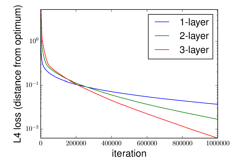
Empirical Evidence: Acceleration with Depth

Comparison of gradient descent on a linear regression task with $\ell_p$ loss. (Fig 3 from Arora et al. 2018)

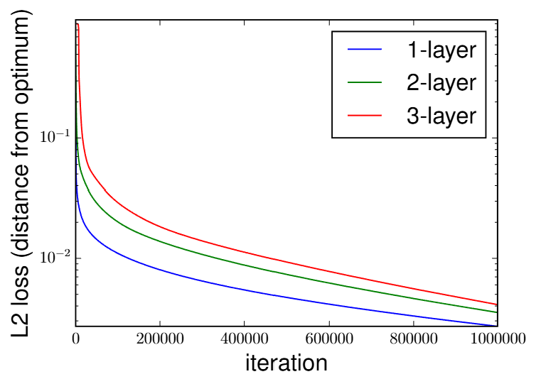
• Left ($\ell_2$ loss): Increasing depth slightly *slows down* convergence, consistent with prior work.
• Right ($\ell_4$ loss): Increasing depth provides a **massive acceleration**, outperforming the shallow model significantly.

The End-to-End Update Rule

Let $W_e = W_N W_{N-1} \cdots W_1$ be the end-to-end matrix. The paper shows that its gradient flow dynamics can be written purely in terms of $W_e$ itself.

The standard gradient $\nabla\mathcal{L}(W_e)$ is pre-multiplied and post-multiplied by fractional matrix powers of $W_e W_e^T$ and $W_e^T W_e$.

A Geometric Interpretation

The complex update rule from Theorem 1 seems arbitrary. But it has a beautiful geometric meaning, unifying it with the concepts from our last lecture.

Let's define the linear preconditioning operator from Theorem 1 as $A_{N,W_e}$: \[ A_{N,W_e}(Z) = \sum_{k=1}^{N} (W_e W_e^T)^{\frac{N-k}{N}} Z (W_e^T W_e)^{\frac{k-1}{N}} \] So the dynamics are $\dot{W}_e = -A_{N,W_e} (E'(W_e))$, where $E'(W_e) = \nabla\mathcal{L}(W_e)$ is the standard Euclidean gradient.

A Geometric Interpretation

The complex update rule from Theorem 1 seems arbitrary. But it has a beautiful geometric meaning, unifying it with the concepts from our last lecture.

Let's define the linear preconditioning operator from Theorem 1 as $A_{N,W_e}$: \[ A_{N,W_e}(Z) = \sum_{k=1}^{N} (W_e W_e^T)^{\frac{N-k}{N}} Z (W_e^T W_e)^{\frac{k-1}{N}} \] So the dynamics are $\dot{W}_e = -A_{N,W_e} (E'(W_e))$, where $E'(W_e) = \nabla\mathcal{L}(W_e)$ is the standard Euclidean gradient.

A Geometric Interpretation

The complex update rule from Theorem 1 seems arbitrary. But it has a beautiful geometric meaning, unifying it with the concepts from our last lecture.

Let's define the linear preconditioning operator from Theorem 1 as $A_{N,W_e}$: \[ A_{N,W_e}(Z) = \sum_{k=1}^{N} (W_e W_e^T)^{\frac{N-k}{N}} Z (W_e^T W_e)^{\frac{k-1}{N}} \] So the dynamics are $\dot{W}_e = -A_{N,W_e} (E'(W_e))$, where $E'(W_e) = \nabla\mathcal{L}(W_e)$ is the standard Euclidean gradient.

Under this specific metric, the complicated dynamics of Theorem 1 become a simple and natural Riemannian gradient flow:

Interpreting the Dynamics (Single Output Case)

For the special case of a single output ($k=1$), the preconditioning scheme simplifies to a more intuitive form.

Interpreting the Dynamics (Single Output Case)

For the special case of a single output ($k=1$), the preconditioning scheme simplifies to a more intuitive form.

• Adaptive Learning Rate: As the weight vector $\|W_e\|$ grows (moves away from zero init), the effective learning rate increases.

Interpreting the Dynamics (Single Output Case)

For the special case of a single output ($k=1$), the preconditioning scheme simplifies to a more intuitive form.

• Adaptive Learning Rate: As the weight vector $\|W_e\|$ grows (moves away from zero init), the effective learning rate increases.
• Momentum: The gradient is amplified along the direction of the current weight vector $W_e$. Since $W_e$ is the integral of past updates, this promotes movement along the historical trajectory.

Proof of Theorem 1 (N=2 case)

Let's derive the end-to-end dynamics for $W_e = W_2 W_1$. The time derivative is $\dot{W}_e = \dot{W}_2 W_1 + W_2 \dot{W}_1$.

1. Substitute the gradient flow dynamics for each layer: \[ \dot{W}_1 = -\eta W_2^T \nabla\mathcal{L}(W_e) \quad , \quad \dot{W}_2 = -\eta \nabla\mathcal{L}(W_e) W_1^T \]

Proof of Theorem 1 (N=2 case)

Let's derive the end-to-end dynamics for $W_e = W_2 W_1$. The time derivative is $\dot{W}_e = \dot{W}_2 W_1 + W_2 \dot{W}_1$.

1. Substitute the gradient flow dynamics for each layer: \[ \dot{W}_1 = -\eta W_2^T \nabla\mathcal{L}(W_e) \quad , \quad \dot{W}_2 = -\eta \nabla\mathcal{L}(W_e) W_1^T \]
2. Plug these into the expression for $\dot{W}_e$: \[ \dot{W}_e = (-\eta \nabla\mathcal{L}(W_e) W_1^T) W_1 + W_2 (-\eta W_2^T \nabla\mathcal{L}(W_e)) \]

Proof of Theorem 1 (N=2 case)

Let's derive the end-to-end dynamics for $W_e = W_2 W_1$. The time derivative is $\dot{W}_e = \dot{W}_2 W_1 + W_2 \dot{W}_1$.

1. Substitute the gradient flow dynamics for each layer: \[ \dot{W}_1 = -\eta W_2^T \nabla\mathcal{L}(W_e) \quad , \quad \dot{W}_2 = -\eta \nabla\mathcal{L}(W_e) W_1^T \]
2. Plug these into the expression for $\dot{W}_e$: \[ \dot{W}_e = (-\eta \nabla\mathcal{L}(W_e) W_1^T) W_1 + W_2 (-\eta W_2^T \nabla\mathcal{L}(W_e)) \]
3. Rearrange the terms: \[ \dot{W}_e = -\eta \left( (W_2 W_2^T) \nabla\mathcal{L}(W_e) + \nabla\mathcal{L}(W_e) (W_1^T W_1) \right) \]

Proof of Theorem 1 (N=2 case)

Let's derive the end-to-end dynamics for $W_e = W_2 W_1$. The time derivative is $\dot{W}_e = \dot{W}_2 W_1 + W_2 \dot{W}_1$.

1. Substitute the gradient flow dynamics for each layer: \[ \dot{W}_1 = -\eta W_2^T \nabla\mathcal{L}(W_e) \quad , \quad \dot{W}_2 = -\eta \nabla\mathcal{L}(W_e) W_1^T \]
2. Plug these into the expression for $\dot{W}_e$: \[ \dot{W}_e = (-\eta \nabla\mathcal{L}(W_e) W_1^T) W_1 + W_2 (-\eta W_2^T \nabla\mathcal{L}(W_e)) \]
3. Rearrange the terms: \[ \dot{W}_e = -\eta \left( (W_2 W_2^T) \nabla\mathcal{L}(W_e) + \nabla\mathcal{L}(W_e) (W_1^T W_1) \right) \]
4. Using the identities for the N=2 case, $W_2 W_2^T = (W_e W_e^T)^{1/2}$ and $W_1^T W_1 = (W_e^T W_e)^{1/2}$:

This matches the general formula from Theorem 1 for $N=2$.

Deriving the Preconditioner (1/3): SVD Setup

How do we derive the fractional powers for $N>2$? Let's analyze $N=3$. Let the SVD of each layer be $W_j = U_j \Sigma_j V_j^T$.

• Balance Invariants: $W_2^T W_2 = W_1 W_1^T$
Hence, their spectra are equal as well $\implies$ $W_1$ and $W_2$ have the same set of singular values.

Deriving the Preconditioner (1/3): SVD Setup

How do we derive the fractional powers for $N>2$? Let's analyze $N=3$. Let the SVD of each layer be $W_j = U_j \Sigma_j V_j^T$.

• Balance Invariants: $W_2^T W_2 = W_1 W_1^T$
Hence, their spectra are equal as well $\implies$ $W_1$ and $W_2$ have the same set of singular values.
• In terms of Polar decomposition, the balance equation implies: \[P_2 = W_2^T W_2 = W_1W_1^T = R_1 \] Hence, $V_2$ (an eigenbasis of $P_2$) and $U_1$ (an eigenbasis of $R_1$) can be chosen to be equal. Therefore, we get the SVD decompositions: \[W_2 = U_2 \Sigma V_2^T \text{ and } W_1 = V_2 \Sigma V_1^T\]

Deriving the Preconditioner (1/3): SVD Setup

How do we derive the fractional powers for $N>2$? Let's analyze $N=3$. Let the SVD of each layer be $W_j = U_j \Sigma_j V_j^T$.

• Balance Invariants: $W_2^T W_2 = W_1 W_1^T$
Hence, their spectra are equal as well $\implies$ $W_1$ and $W_2$ have the same set of singular values.
• In terms of Polar decomposition, the balance equation implies: \[P_2 = W_2^T W_2 = W_1W_1^T = R_1 \] Hence, $V_2$ (an eigenbasis of $P_2$) and $U_1$ (an eigenbasis of $R_1$) can be chosen to be equal. Therefore, we get the SVD decompositions: \[W_2 = U_2 \Sigma V_2^T \text{ and } W_1 = V_2 \Sigma V_1^T\]
• Similarly using the balance equation for $W_2$ and $W_3$, we get the SVDs \[W_3 = U_3 \Sigma V_3^T \text{ , } W_2 = V_3 \Sigma V_2^T \text{ and } W_1 = V_2 \Sigma V_1^T\]

Derivation (2/3): Simplifying the Product

Let's express the end-to-end matrix $W_e = W_3 W_2 W_1$ using the SVDs and the relationships we found.

Derivation (3/3): Final Identities

From $W_e = U_3 \Sigma^3 V_1^T$, we can identify the SVD components of $W_e = U_e \Sigma_e V_e^T$ as:

Now we can express the individual layer terms using the end-to-end SVD components.

• For the last layer, $W_3 W_3^T = U_3 \Sigma^2 U_3^T$. Since $U_3 = U_e$ and $\Sigma = \Sigma_e^{1/3}$: \[ W_3 W_3^T = U_e (\Sigma_e^{1/3})^2 U_e^T = (U_e \Sigma_e U_e^T)^{2/3} = (W_e W_e^T)^{2/3} \]
• For the first layer, $W_1^T W_1 = V_1 \Sigma^2 V_1^T$. Using $\Sigma = \Sigma_e^{1/3}$ and $V_1 = V_e$: \[ W_1^T W_1 = V_1 (\Sigma_e^{1/3})^2 V_1^T = (V_e^T \Sigma_e V_e)^{2/3} = (W_e^T W_e)^{2/3} \]

This is where the fractional powers in Theorem 1 come from. The exponent is $\frac{N-j}{N}$ for post-multiplication and $\frac{j-1}{N}$ for pre-multiplication.

How This Leads to Acceleration (1/4): Setup

We analyze a simple, ill-conditioned linear regression problem with $\ell_4$ loss and $N=2$ overparameterization.

• Data: Two points, $([1,0], y_1)$ and $([0,1], y_2)$.
• Loss: $L(w_1, w_2) = \frac{1}{4}(w_1 - y_1)^4 + \frac{1}{4}(w_2 - y_2)^4$.
• Ill-Conditioning: Assume $|y_1| \gg |y_2| \approx 1$.
• Initialization: Near-zero weights, $w_1^{(0)}=\epsilon_1, w_2^{(0)}=\epsilon_2$, with $\epsilon_2/\epsilon_1 \approx y_2/y_1$.

Reference: GD Convergence Bounds

For a general convex function $L(w)$ with an L-Lipschitz continuous gradient, the following bounds provide the context for our analysis:

How This Leads to Acceleration (2/4): Standard GD

The standard gradient descent update for each coordinate is decoupled:

How This Leads to Acceleration (2/4): Standard GD

The standard gradient descent update for each coordinate is decoupled:

• To avoid divergence, the learning rate $\eta$ is limited by the coordinate with the largest gradient, which is $w_1$. The stability condition requires: \[ \eta < \frac{2}{(w_1-y_1)^2} \approx \frac{2}{y_1^2} \]

How This Leads to Acceleration (2/4): Standard GD

The standard gradient descent update for each coordinate is decoupled:

• To avoid divergence, the learning rate $\eta$ is limited by the coordinate with the largest gradient, which is $w_1$. The stability condition requires: \[ \eta < \frac{2}{(w_1-y_1)^2} \approx \frac{2}{y_1^2} \]
• This very small learning rate, dictated by $y_1$, is then applied to the update for $w_2$.
• The convergence for $w_2$ is extremely slow. The error $\Delta_2 = w_2 - y_2$ shrinks by a factor of approximately $(1 - \eta y_2^2)$ at each step, which is very close to 1.

How This Leads to Acceleration (3/4): Overparameterized GD

For $N=2$, the discrete update rule for a single output network is:

Let's analyze the first iteration ($t=0$). The gradients are $\nabla_1 \approx -y_1^3$ and $\nabla_2 \approx -y_2^3$.

The update for each component is:

Using the condition $\epsilon_2/\epsilon_1 \approx y_2/y_1 \ll 1$, we have $\sqrt{\epsilon_1^2+\epsilon_2^2} \approx \epsilon_1$. This simplifies the updates to:

How This Leads to Acceleration (4/4): The Punchline

With the update rules $w_1^{(1)} \approx \epsilon_1 + \eta(2\epsilon_1 y_1^3)$ and $w_2^{(1)} \approx \epsilon_2 + \eta(\epsilon_1 y_2^3 + \epsilon_2 y_1^3)$:

1. Choose $\eta$: We can now choose a large learning rate for $w_1$ to make it converge in one step. Let $\eta = \frac{1}{2\epsilon_1 y_1^2}$. This gives $w_1^{(1)} \approx \epsilon_1 + \frac{1}{2\epsilon_1 y_1^2}(2\epsilon_1 y_1^3) \approx y_1$.
2. Analyze $w_2$ update: With this $\eta$, the update for $w_2$ becomes: \[ w_2^{(1)} \approx \epsilon_2 + \frac{1}{2\epsilon_1 y_1^2} (\epsilon_1 y_2^3 + \epsilon_2 y_1^3) \approx \frac{y_2^3}{2 y_1^2} + \frac{\epsilon_2}{2\epsilon_1}y_1 \approx \frac{y_2}{2} \] (The first term is negligible, and we used $\epsilon_2/\epsilon_1 \approx y_2/y_1$).
3. Compare Rates: In one step, $w_2$ has moved halfway to its target $y_2$. The effective learning rate for $w_2$ after $w_1$ converges is $\eta_{OP} \approx \frac{1}{2\epsilon_1 y_1}$. The speedup is: \[ \frac{\eta_{OP}}{\eta_{GD}} > \frac{1/(2\epsilon_1 y_1)}{2/y_1^2} = \frac{y_1}{4\epsilon_1} \gg 1 \]

Overparameterization allows the large coordinate to "lend" its scale to accelerate the small coordinate.